Solving Generalized Assignment Problem using Branch-And-Price
Table of Contents
Generalized Assignment Problem
One of the best known and widely researched problems in combinatorial optimization is Knapsack Problem:
- given a set of items, each with its weight and value,
- select a set of items maximizing total value
- that can fit into a knapsack while respecting its weight limit.
The most common variant of a problem, called 0-1 Knapsack Problem can be formulated as follows:
\[\begin{array}{lrcl} \max & \displaystyle\sum_{i=1}^{m} v_i x_i &\\ \textrm{subject to} & \displaystyle \sum_{i=1}^{m} w_i x_i & \le & W\\ & x_i & \in & \{0, 1\} \\ \end{array}\]where
- \(m\) - number of items;
- \(x_i\) - binary variable indicating whether item is selected;
- \(v_i\) - value of each items;
- \(w_i\) - weight of each items;
- \(W\) - maximum weight capacity.
As often happens in mathematics, or science in general, an obvious question to ask is how the problem can be generalized. One of generalization is Generalized Assignment Problem. It answers question - how to find a maximum profit assignment of \(m\) tasks to \(n\) machines such that each task (\(i=0, \ldots, m\)) is assigned to exactly one machine (\(j=1, \ldots, n\)), and one machine can have multiple tasks assigned to subject to its capacity limitation. Its standard formulation is presented below:
\[\begin{array}{lrclll} \max & \displaystyle\sum_{i=0}^{m} \sum_{j=1}^{n} v_{ij} x_{ij} & & &\\ \textrm{subject to} & \displaystyle \sum_{j=1}^{n} x_{ij} & =& 1 & i=1, \ldots, m & \textrm{(task assignment)} \\ & \displaystyle \sum_{i=1}^{m} w_{ij} x_{ij} & \le & c_j & j=1, \ldots, n & \textrm{(machine capacity)} \\ & x_{ij} & \in & \{0, 1\} & & \\ \end{array}\]where
- \(n\) - number of machines;
- \(m\) - number of tasks;
- \(x_{ij}\) - binary variable indicating whether task \(i\) is assigned to machine \(j\);
- \(v_{ij}\) - value/profit of assigning task \(i\) to machine \(j\);
- \(w_{ij}\) - weight of assigning task \(i\) to machine \(j\);
- \(c_j\) - capacity of machine \(j\).
Branch-and-price
Branch-and-price is generalization of branch-and-bound method to solve integer programs (IPs),mixed integer programs (MIPs) or binary problems. Both branch-and-price, branch-and-bound, and also branch-and-cut, solve LP relaxation of a given IP. The goal of branch-and-price is to tighten LP relaxation by generating a subset of profitable columns associated with variables to join the current basis.
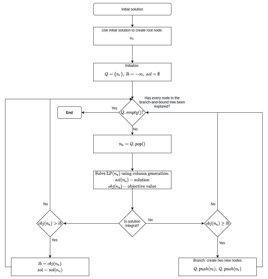
Branch-and-price builds at the top of branch-and-bound framework. It applies column generation priori to branching. Assuming maximization problem, branching occurs when:
- Column Generation is finished (i.e. no profitable columns can be found).
- Objective value of the current solution is greater than best lower bound.
- The current solution does not satisfy integrality constraints.
However, if only first two conditions are met but not the third one, meaning the current solution satisfies integrality constraints, then the best solution and lower bound are updated (lower bound is tightened) with respectively the current solution and its objective value.
The crucial element needed to apply branch-and-price successfully is to find branching scheme. It is tailored to specific problem to make sure that it does not destroy problem structure and can be used in pricing subproblem to effectively generate columns that enter Restricted Master Problem (RMP) while respecting branching rules .
Below is flow diagram describing branch-and-price method:
Dantzig-Wolfe decomposition
The successful application B&P depends on tight/strong model formulation. Model formulation is considered tight if solution of its LP relaxation satisfies (frequently) integrality constraints. One of structured approaches to come up with such a formulation is to use Dantzig-Wolfe Decomposition technique. We will see example of it applied to Generalized Assignment Problem (GAP).
A standard formulation was described above. Now, let’s try to reformulate problem. Let
\[S_j = \{\mathbf{x}: \mathbf{x} \in \{0, 1\}^{m} \wedge \mathbf{x}^T \mathbf{w}_j \le c_j \}\]be a set containing all feasible solutions to Knapsack problem for \(j\)-th machine. Clearly, \(S_j\) contains finite number of points, so \(S_j = \{ \mathbf{z}_j^1, \ldots, \mathbf{z}_j^{K_j} \}\), where \(\mathbf{z}_j^k \in \{0, 1\}^{m}\). You can think about \(\mathbf{z}_j^k \in \{0, 1\}^{m}\) as 0-1 encoding of tasks that form \(k\)-th feasible solution for machine \(j\). Now, let \(S = \{ \mathbf{z}_1^1, \ldots, \mathbf{z}_1^{K_1}, \ldots, \mathbf{z}_n^1, \ldots, \mathbf{z}_n^{K_n} \}\) be a set of all feasible solution to GAP. It, potentially, contains a very large number of elements. Then, every point \(x_{ij}\) can be expressed by the following convex combination:
\[\begin{array}{rcll} x_{ij} & = & \displaystyle \sum_{k=1}^{K_j} z_{ij}^k \lambda_j ^k & \\ \displaystyle \sum_{k=1}^{K_j} \lambda_j ^k & = & 1, & j=1,\ldots, n \\ \lambda_i ^k & \in & \{0, 1\} & j=1,\ldots, n, \ k = 1, \ldots, K_j \end{array}\]where \(z_{ij}^k \in \{0, 1\}\), and \(z_{ij}^k = 1\) iff task \(i\) is assigned to machine \(j\) in \(k\)-th feasible solution for the machine.
Now, let’s use this representation to reformulate GAP:
\[\begin{array}{lrclll} \max &\displaystyle \sum_{j=1}^{n}\sum_{k=0}^{K_j} \left( v_{ij} z_{ij}^k \right) \lambda_j ^k & & &\\ \textrm{subject to} & \displaystyle \sum_{j=1}^{n}\sum_{k=0}^{K_j} z_{ij}^k \lambda_j ^k & = & 1 & i=1, \ldots, m & \textrm{(task assignment)} \\ & \displaystyle \sum_{k=0}^{K_j} \lambda_j ^k & = & 1 & j=1, \ldots, n & \textrm{(convexity)} \\ \end{array}\]Note that we do not need capacity restrictions as they are embedded into definition of feasible solution for machine \(j\).
Now that we have formulation that is suitable for column generation, let’s turn our attention to it.
Column generation
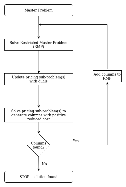
Column generation is another crucial component of branch-and-price. There are many great resources devoted to column generation so I will mention only core points:
- Column generation is useful when a problem’s pool of feasible solutions contains many elements but only small subset will be present in the optimal solution.
- There exists subproblem (called often pricing problem) that can be used to effectively generate columns that should enter RMP.
- Column generation starts with initial feasible solution.
- Pricing subproblem objective function is updated with dual of the current solution.
- Columns with positive reduced cost, in case of maximization problem, enter problem.
- Procedure continues until such columns exist.
Below is flow diagram describing column generation method:
Implementation
Let’s see how one can approach implementation of B&P to solve Generalized Assignment Problem. Below is discussion about main concepts and few code excerpts, a repository containing all code can be found on github.
@dataclass(frozen=True)
class GeneralAssignmentProblem:

    num_tasks: int
    num_machines: int
    weights: np.ndarray  # shape: num_machines x num_tasks
    profits: np.ndarray  # shape: num_machines x num_tasks
    capacity: np.ndarray  # shape: num_machines x num_tasks
An example of problem instance taken from [1] is:
num_machines = 2
num_tasks = 3
profits = np.array([
    [10, 7, 5],
    [6, 8, 11]
])

weights = np.array([
    [9, 6, 3],
    [5, 7, 9]
])

capacity = np.array([11, 18])
Standalone model
It is always good idea to have a reference simple(r) implementation that can be used to validate our results using more sophisticated methods. In our case it is based on standard problem formulation. Implementation can be found in repo by checking classes GAPStandaloneModelBuilder and GAPStandaloneModel. Formulation for a problem instance presented above looks as follows:
\ Model gap_standalone_model
\ LP format - for model browsing. Use MPS format to capture full model detail.
Maximize
  10 task_0_machine_0 + 6 task_0_machine_1
   + 7 task_1_machine_0 + 8 task_1_machine_1
   + 5 task_2_machine_0 + 11 task_2_machine_1
Subject To
 task_assignment_0: task_0_machine_0 + task_0_machine_1 = 1
 task_assignment_1: task_1_machine_0 + task_1_machine_1 = 1
 task_assignment_2: task_2_machine_0 + task_2_machine_1 = 1
 machine_capacity_0: 9 task_0_machine_0 + 6 task_1_machine_0 + 3 task_2_machine_0 <= 11
 machine_capacity_1: 5 task_0_machine_1 + 7 task_1_machine_1 + 9 task_2_machine_1 <= 18
Bounds
Binaries
 task_0_machine_0 task_0_machine_1
 task_1_machine_0 task_1_machine_1
 task_2_machine_0 task_2_machine_1
End
Now let’s try to examine building blocks of B&P to discus main part at the end, once all the puzzles are there.
Initial solution
To start column generation process, we need to have an initial solution. One possible way to derive it is to use two-phase Simplex method. In first step, you add slack variables to each constraint and set objective function as their sum. Then you minimize the problem. If your solution has objective value \(0\), then first of all you have initial solution and you know that your problem is feasible. In case you end up with positive value for any of slack variables, you can conclude that the problem is infeasible. You can stop here.
I took a different approach and came up with simple heuristic that generate initial solution. I have not analyzed it thoroughly so I am not sure if it is guaranteed to always return feasible solution if one exists. Its idea is quite simple:
- Solves a sequence of minimum weight matching problems for bipartite graph:
- Construct bipartite graph defined as \(G=(V, A)\), where \(V = T \cup M\) – \(T\) is set of tasks and obviously \(M\) is set of machines. There exists arc \(a = (t, m)\) if \(w_{tm} \le rc_{m}\), where \(rc_{m}\) is remaining capacity for machine \(m\). Initially remaining capacity is equal to capacity of machine and with each iteration, and assignment of task to machine it is being update. If \(\vert A \vert = 0\), then stop.
- Solve a minimum weight matching problem.
- Update assignments – say that according to solution task \(t_0\) should be assigned to machine \(m_0\), then \(\overline{rc}_{m_0} = rc_{m_0} - w_{t_0 m_0}\).
- For every unassigned task - \(t_0\):
- Find a machine where task is contributing with the lowest weight – say machine \(m_0 = \arg\min \{ m: w_{t_0 m} \}\).
- Free up remaining capacity so there is enough space for \(t_0\) on machine \(m_0\). Any tasks that were de-assigned in a process are added to pool of unassigned tasks.
- Repeat until there are no unassigned tasks.
See details on github.
Branching rule
As we said before the most important piece needed to implement B&P is branching rules which does not destroy structure of subproblem. Let’s consider non-integral solution to RMP. Given convexity constraint it means that there exists machine \(j_0\) and at least two, and for sake of example say exactly two, \(0 < \lambda_{j_0} ^{k_1} < 1\) and \(0 < \lambda_{j_0} ^{k_2} < 1\) such that \(\lambda_{j_0} ^{k_1} + \lambda_{j_0} ^{k_2} = 1\). Since with each of \(\lambda\)s is connected different assignment (set of tasks), then it leads us to a conclusion that there exists task \(i_0\) such that \(x_{i_0 j_0} < 1\) expressed in variables from the original formulation. Now, let’s use this information to formulate branching rule:
- left child node: a task \(i_0\) must be assigned to a machine \(j_0\).
- right child node: a task \(i_0\) cannot be assigned to a machine \(j_0\).
We can say that branching is based on \(x_{ij}\) from standard formulation. And it can be represented by:
@dataclasses.dataclass(frozen=True)
class BranchingRule:
    task: int
    machine: int
    assigned: bool
Note that we can use the branching rule to easily to filter out initial columns for each node that do not satisfy those conditions:
- left child node: column representing assignment of tasks, \(T_j\), to machine \(j\) is kept if:
- \(j = j_0\) and task \(i_0 \in T_{j_0}\), or
- \(j \neq j_0\) and task \(i_0 \notin T_{j}\).
- right childe node: column representing assignment of tasks, \(T_j\), to machine \(j\) is filtered out if:
- \(j = j_0\) and task \(i_0 \in T_{j_0}\).
See on github.
Based on the same principle, subproblem’s pool of feasible solution are created - i.e. on left child node:
- knapsack subproblem for machine \(j_0\) – variable representing task \(i_0\) is forced to be \(1\).
- knapsack subproblem for machine \(j \neq j_0\) – variable representing task \(i_0\) is forced to be \(0\).
Similarly for right childe node. See on github.
Column generation
Below is an outline of main loop of column generation. It is an implementation of flow diagram from above so I will not spend too much time describing it. The only part maybe worth commenting is stop_due_to_no_progress - it evaluates whether column generation did not make any progress in last \(k\)-iterations and it should be stop.
class BranchNode:

    def __init__(self, ...):
        # ...
        self._rmp = grb.Model(f'GAP_RMP_{self.id}')


    def _solve_using_column_generation(self):
        # ...

        while True:
            # ...

            self._rmp.optimize()

            if stop_due_to_no_progress():
                break

            columns_added = self._solve_knapsack_subproblems()
            if not columns_added:
                break

    def _solve_knapsack_subproblems(self) -> bool:

        try:
            # obtain duals associated with tasks, solution might be infeasible
            # but duals will be returned
            task_duals = [row.Pi for _, row in self.task_to_assignment_constraint.items()]
            machine_duals = [row.Pi for _, row in self.machine_to_assignment_constraint.items()]
        except AttributeError:
            # no dual information
            return False

        subproblem_builder = SubproblemBuilder(gap_instance=self.gap_instance)

        columns_added = False
        for machine_id in range(self.gap_instance.num_machines):

            machine_dual = machine_duals[machine_id]

            # building knapsack subproblem using dual information
            subproblem = subproblem_builder.build(machine_id=machine_id,
                                                  machine_dual=machine_dual,
                                                  task_duals=task_duals,
                                                  branching_rules=self.branching_rules)

            subproblem.solve()
            subproblem_objective_value = subproblem.objective_value()

            # are there any columns with positive reduced cost?
            # only those can improve RMP solution
            if subproblem_objective_value is None or subproblem_objective_value <= 0:
                continue

            columns_added = True

            for machine_schedule in subproblem.all_solutions():
                self._add_column_to_rmp(machine_schedule)

        return columns_added
Now, let’s see how constructing subproblems, solving them and then adding back column(s) to RMP looks like. We have as many subproblems as machines. Once a solution is available, we check whether it has positive reduced cost. A solution to knapsack problem corresponds to column in RMP. So if the column with positive reduced cost was identified and added, then new iteration of column generation will be executed. Gurobi allows to query information about all other identified solutions, so we can utilize this feature and add all columns that have the same objective value as optimal solution, potentially adding more than one column and hoping it will positively impact solution time.
class BranchNode:

    # ...

    def _solve_knapsack_subproblems(self) -> bool:

        try:
            # obtain duals associated with tasks, solution might be infeasible
            # but duals will be returned
            task_duals = [row.Pi for _, row in self.task_to_assignment_constraint.items()]
            machine_duals = [row.Pi for _, row in self.machine_to_assignment_constraint.items()]
        except AttributeError:
            # no dual information
            return False

        subproblem_builder = SubproblemBuilder(gap_instance=self.gap_instance)

        columns_added = False
        for machine_id in range(self.gap_instance.num_machines):

            machine_dual = machine_duals[machine_id]

            # building knapsack subproblem using dual information
            subproblem = subproblem_builder.build(machine_id=machine_id,
                                                  machine_dual=machine_dual,
                                                  task_duals=task_duals,
                                                  branching_rules=self.branching_rules)

            subproblem.solve()
            subproblem_objective_value = subproblem.objective_value()

            # are there any columns with positive reduced cost?
            # only those can improve RMP solution
            if subproblem_objective_value is None or subproblem_objective_value <= 0:
                continue

            columns_added = True

            for machine_schedule in subproblem.all_solutions():
                self._add_column_to_rmp(machine_schedule)

        return columns_added
Note that each subproblem is independent so in principle they could be solved in parallel. However due to Python Global Interpreter Lock (GIL) that prevent CPU-bounded threads to run in parallel, they are solved sequentially. Additionally depending on your Gurobi license, you might not be allowed to solve all those models in parallel even if Python would allow it.
Below you can find example of one of the RMPs:
\ Model GAP_RMP_2
\ LP format - for model browsing. Use MPS format to capture full model detail.
Maximize
  26 machine_0_tasks_1_2_4_5 + 20 machine_0_tasks_0_2_4 + 27 machine_0_tasks_0_1_3_4
  + 29 machine_0_tasks_0_1_2_4 + 19 machine_0_tasks_0_4_5
  + 15 machine_1_tasks_2_3_5 + 9 machine_1_tasks_5_6 + 13 machine_1_tasks_0_1_3
  + 13 machine_1_tasks_2_6

Subject To
 task_assignment_0: machine_0_tasks_0_2_4 + machine_0_tasks_0_4_5
   + machine_0_tasks_0_1_3_4 + machine_0_tasks_0_1_2_4
   + machine_1_tasks_0_1_3  = 1
 task_assignment_1: machine_0_tasks_1_2_4_5 + machine_0_tasks_0_1_3_4
   + machine_0_tasks_0_1_2_4   + machine_1_tasks_0_1_3 = 1
 task_assignment_2: machine_0_tasks_1_2_4_5 + machine_0_tasks_0_2_4
    + machine_0_tasks_0_1_2_4
    + machine_1_tasks_2_3_5 + machine_1_tasks_2_6 = 1
 task_assignment_3: machine_1_tasks_2_3_5 + machine_1_tasks_0_1_3
   + machine_0_tasks_0_1_3_4 = 1
 task_assignment_4: machine_0_tasks_1_2_4_5 + machine_0_tasks_0_2_4
   + machine_0_tasks_0_4_5 + machine_0_tasks_0_1_3_4
   + machine_0_tasks_0_1_2_4 = 1
 task_assignment_5: machine_0_tasks_1_2_4_5 + machine_0_tasks_0_4_5
   + machine_1_tasks_2_3_5 + machine_1_tasks_5_6 = 1
 task_assignment_6: machine_1_tasks_5_6 + machine_1_tasks_2_6 = 1
 convexity_machine_0: machine_0_tasks_1_2_4_5 + machine_0_tasks_0_2_4
   + machine_0_tasks_0_4_5 + machine_0_tasks_0_1_3_4
   + machine_0_tasks_0_1_2_4 = 1
 convexity_machine_1: machine_1_tasks_2_3_5 + machine_1_tasks_5_6
   + machine_1_tasks_0_1_3 + machine_1_tasks_2_6 = 1
Bounds
End
and subproblem with dual information passed:
\ Model GAP_Subproblem
\ LP format - for model browsing. Use MPS format to capture full model detail.
Maximize
  4.333333333333333 task_0_machine_0 + 3.833333333333333 task_1_machine_0
   + 0.5 task_2_machine_0 - 0.3333333333333339 task_3_machine_0
   + 4.333333333333334 task_4_machine_0 + 3.5 task_5_machine_0
   + 6.166666666666666 task_6_machine_0 - 12.16666666666667 Constant
Subject To
 machine_capacity_0: 4 task_0_machine_0 + task_1_machine_0
   + 2 task_2_machine_0 + task_3_machine_0 + 4 task_4_machine_0
   + 3 task_5_machine_0 + 8 task_6_machine_0 <= 11
Bounds
 Constant = 1
Binaries
 task_0_machine_0 task_1_machine_0 task_2_machine_0 task_3_machine_0
 task_4_machine_0 task_5_machine_0 task_6_machine_0
End
Branch-and-Price
Now that we have all building blocks prepared, then let’s turn our attention back to B&P.
class GAPBranchAndPrice:

    def solve(self):
        queue: Queue[BranchNode] = Queue([
            self._create_root_node()
        ])

        # ...

        while not queue.is_empty():

            current_node = queue.pop()

            current_node.solve()

            if not current_node.is_feasible():
                continue

            if current_node.has_integer_solution():
                update_best_found_solution()
            else:
                obj = current_node.objective_value()
                if nodes := self._branch(current_node, mip_lb):
                    include_nd, exclude_nd = nodes
                    queue.push(include_nd)
                    queue.push(exclude_nd)

        best_solution_node.report_integer_solution()

    @classmethod
    def _branch(cls, node: BranchNode, mip_lb: float) -> Optional[Tuple[BranchNode, BranchNode]]:

        if mip_lb is not None and node.objective_value() <= mip_lb:
            # in case node's LP value is lower than
            # so far found MIP LB, then whole tree rooted at node
            # can be discarded
            return None

        if node.objective_value() == math.nan:
            # Model after branching might become infeasible
            return None

        # based on current solution obtain id of task and machine
        machine, task = node.machine_task_to_branch_on()

        # create two branching rules
        exclude_branching = BranchingRule(task, machine, assigned=False)
        include_branching = BranchingRule(task, machine, assigned=True)

        # current branching rules
        br_rls = node.branching_rules

        exclude_nd = BranchNode(
            node.gap_instance,
            copy.deepcopy(br_rls) + [exclude_branching],
            copy.deepcopy(node.get_machine_schedules()),
        )

        include_nd = BranchNode(
            node.gap_instance,
            copy.deepcopy(br_rls) + [include_branching],
            copy.deepcopy(node.get_machine_schedules()),
        )

        return exclude_nd, include_nd
Summary
In the blog post, Branch-and-Price technique for solving MIP was explained. An example of applying B&P for Generalized Assignment Problem was presented. The solution approach used Python as programming language and Gurobi as solver.
References
[1] Der-San Chen, Robert G. Batson, Yu Dang (2010), Applied Integer Programming - Modeling and Solution, Willey.
[2] Lasdon, Leon S. (2002), Optimization Theory for Large Systems, Mineola, New York: Dover Publications.
[3] Cynthia Barnhart, Ellis L. Johnson, George L. Nemhauser, Martin W. P. Savelsbergh, Pamela H. Vance, (1998) Branch-and-Price: Column Generation for Solving Huge Integer Programs. Operations Research 46(3):316-329.